Blog
Mehtaab Sawhney wins Clay Research Fellowship
January 25, 2024

Congratulation to Mehtaab for this prestigious and highly deserved honor!
Here is the award citation.
Papers by MIT combinatorialists—Fall 2023
December 22, 2023
As we near the end of the year, I’m delighted to showcase and celebrate a selection of recent papers by the talented combinatorialists at MIT, especially those by students and postdocs. These papers reflect the culmination of their hard work, dedication, and innovative problem solving. For each paper, I’ll offer a concise summary, and I encourage you to read the papers to learn more about the beautiful mathematics within.
Additive Combinatorics
- Effective bounds for Roth’s theorem with shifted square common difference
Sarah Peluse, Ashwin Sah, Mehtaab Sawhney
This paper proves the first quantitative upper bound on an interesting special case of the polynomial Szemerédi theorem. Specifically, it shows that the maximum size of a subset of \(\{1, \dots, N\}\) avoiding the pattern $x, x + y^2 - 1, x + 2(y^2 - 1)$ is at most $N / \log \log \cdots \log N$, with at most a constant number of logs. This special case was highlighted by Green.
This paper introduces a new perspective on the polynomial method, unifying various earlier arguments in the field that initially looked quite distinct.
- Size of the largest sum-free subset of $[n]^3$, $[n]^4$, and $[n]^5$
Saba Lepsveridze, Yihang Sun
This paper determines the density of the largest sum-free subset of the lattice cube \(\{1, \dots, n\}^d\) for $d = 3, 4, 5$, resolving a conjecture of Cameron and Aydinian in these dimensions.
- $(n,k)$-Besicovitch sets do not exist in $\mathbb{Z}_p^n$ and $\hat{\mathbb{Z}}^n$ for $k \ge 2$
Manik Dhar
This paper proves that over the $p$-adics and profinite integers, any set which contains a 2-flat in every direction must have positive measure. This extends earlier results on discrete Kakeya.
This paper shows that the maximum size of a subset of \(\{1, \dots, N\}\) without a 5-term arithmetic progression is at most $N \exp ( -(\log\log N)^c)$, improving Gowers’ longstanding $N (\log\log N)^{-c}$ bound.
Discrete Geometry
This paper shows that every subset of a sphere avoiding an orthonormal basis has measure at most $c_0$, where $c_0 < 1$ is some absolute constant independent of the dimension.
- Uniacute spherical codes
Saba Lepsveridze, Aleksandre Saatashvili, Yufei Zhao
Extending earlier work on equiangular lines, this paper studies the maximum number of unit vectors in \(\mathbb{R}^d\) whose pairwise inner products lie in some given \(L \subseteq [-1,1)\), specifically in the case where \(L = [-1, -\beta] \cup \{\alpha\}\). The main result determines all such $L$ where the “uniform bound” of Balla, Dräxler, Keevash, and Sudakov is tight.
Random Matrix Theory
Let $A_n$ be an $n \times n$ random matrix whose entries are independent Bernoulli random variables with probability $d/n$ (where $d > 0$ is a constant). This paper shows that the spectral distribution \(\mu_{A_n}\) converges in probability to some limiting distribution \(\mu_d\) on the complex plane.
Random Graphs
This paper studies the structure of a sparse Erdős–Rényi random graph conditioned on a lower tail subgraph count event. When the subgraph count is conditioned to be slightly below expectation, the typical random graph is shown to be close to another Erdős–Rényi random graph (with lower edge density) in both cut norm and subgraph counts.
[Edit: 12/26/2023 added last entry]
Schildkraut: Equiangular lines and large multiplicity of fixed second eigenvalue
March 6, 2023
I am excited to share and discuss the latest work by an MIT undergraduate senior, Carl Schildkraut, titled Equiangular lines and large multiplicity of fixed second eigenvalue. In his paper, Carl offers new constructions on two related problems:
- equiangular lines,
- graphs with high second eigenvalue multiplicity.
Equiangular lines
In my previous work on equiangular lines (with Zilin Jiang, Jonathan Tidor, Yuan Yao, and Shengtong Zhang) (previously reported on this blog and MIT News), we solved the following problem:
Problem (Equiangular lines with a fixed angle). For a given fixed angle, in sufficiently high dimensions, determine the maximum possible number of lines that can be pairwise separated by the given angle.
The answer can be phrased in terms of the spectral radius order $k(\lambda)$, defined to be the smallest integer $k$ so that there exists a $k$-vertex graph $G$ whose adjacency matrix has top eigenvalue exactly $\lambda$. Furthermore, we define $k(\lambda) = \infty$ if no such graph $G$ exists.
Theorem (Jiang–Tidor–Yao–Zhang–Zhao). For $\alpha \in (0,1)$. Let $\lambda = (1-\alpha)/(2\alpha)$ and let $k(\lambda)$ be its spectral radius order. Then the maximum number $N_\alpha(d)$ of equiangular lines in $\mathbb{R}^d$ with common angle $\arccos \alpha$ satisfies:
(a) If $k(\lambda) < \infty$, then $N_\alpha(d) = \lfloor k(d-1) / (k-1) \rfloor$ for all sufficiently large $d$;
(b) If $k(\lambda) = \infty$, then $N_\alpha(d) = d + o(d)$ as $d \to \infty$.
In particular, this result determines the first order growth rate of $N_\alpha(d)$ for all $\alpha$. Even better, when the spectral radius order is finite, our result determines the answer exactly in all sufficiently large dimensions. (There is a tantalizing open question on how high the dimension needs to be.) However, when the spectral radius order is infinite, our result gives only an asymptotic $d + o(d)$. Can we hope for a more precise answer?
Jiang and Polyanskii conjectured that $N_\alpha(d) = d + O_\alpha(1)$ when $k(\lambda) = \infty$, i.e., the $o(d)$ error term should be at most constant depending on $\lambda$. They verified this conjecture when $\lambda$ is either (a) not a totally real algebraic integer or (b) a totally real algebraic integer that is not the largest among its Galois conjugates. We also reiterated this conjecture in our paper.
Carl Schildkraut’s new paper gives a counterexample to this conjecture.
Theorem (Schildkraut). There exist infinitely many $\alpha$ such that $N_{\alpha}(d) = d + o(d)$ and yet $N_{\alpha}(d) \ge d + \Omega_\alpha(\log \log d)$.
I found this result to be quite surprising. I had expected the opposite to be true.
Second eigenvalue multiplicity
One of the key ingredients in our equiangular lines paper is a bound on the second eigenvalue multiplicity.
Theorem (Jiang-Tidor-Yao-Zhang-Zhao). The adjacency matrix of every connected $n$-vertex graph with maximum degree $\Delta$ has second eigenvalue multiplicity at most $O_\Delta(n/\log \log n)$.
The fact that the second eigenvalue multiplicity is sublinear in the number of vertices plays a crucial role in our solution to the equiangular lines with a fixed angle problem.
The second eigenvalue multiplicity bound leaves many open questions.
How tight is the bound? The quantitative bound is the bottleneck being able to improve the “sufficiently large dimension” part of the equiangular lines result. The $O_\Delta(n/\log\log n)$ bound is still best known (though, see the work of McKenzie–Rasmussen–Srivastava for an improvement to $O_\Delta(n/(\log n)^c)$ in the case of regular graphs). See my work with Milan Haiman, Carl Schildkraut, Shengtong Zhang (previously reported on this blog) for the current best lower bound constructions, giving $\Omega(\sqrt{n /\log n})$.
Here is a question relevant to the equiangular lines problem with a fixed angle (appearing as Question 6.4 in our equiangular lines paper):
Question. Fix $\Delta, \lambda >0$. What is the maximum multiplicity that $\lambda$ as the second eigenvalue of a connected $n$-vertex graph with maximum degree at most $\Delta$?
We suggested the possibility that perhaps the answer is always at most a constant depending on $\Delta$ and $\lambda$. I really thought that the answer should be bounded. Carl’s paper shows otherwise.
Theorem (Schildkraut). For infinitely many values of $\lambda$ and $d$, there exist sequences of connected $d$-regular $n$-vertex graphs whose second eigenvalue is exactly $\lambda$ and has multiplicity at least $\Omega_{d, \lambda}(\log \log n)$.
So now we know that the answer to the earlier question is between $\Omega(\log\log n)$ and $O(n/\log \log n)$. There is still a huge gap.
Carl managed to get his construction many families of $\lambda$, including some with $k(\lambda) = \infty$, which implies his equiangular lines result stated earlier.
Carl’s construction is quite elegant, incorporating several clever ideas in spectral graph theory. One of the ideas used is the 2-lift technique from the seminal Bilu-Linial paper. This is a way to transform a graph into another graph with twice as many vertices and in a way that allows us to control the spectrum.
For Carl’s construction, in order to perform the 2-lift and control the eigenvalues, given a $d$-regular bipartite graph, he needs to select a regular subgraph in a way that is somewhat random. There needs to be enough independent sources of randomness so that he can apply concentration bounds. He does this by, roughly speaking, partitioning the graph into short even cycles, and then for each even cycle, independently choosing one of the two alternating sets of edges.
There is another catch, which is that in order for his concentration bounds to go through, he needs to first make the graph large enough so that the relevant eigenvectors are all somewhat flat. He does this by repeatedly performing the Ramanujan lift from the seminal work of Marcus–Spielman–Srivastava. (Carl doesn’t need the full strength of the MSS result, but why resist applying such a beautiful theorem.)
This is really nice construction. These interesting ideas will surely lead to further developments in spectral graph theory.
Nearly all k-SAT functions are unate
September 19, 2022
The Boolean satisfiability problem, specifically k-SAT, occupies a central place in theoretical computer science. Here is a question that had been open until just now: what does a typical k-SAT function look like? Bollobás, Brightwell, and Leader (2003) initiated the study of this question, and they conjectured that a typical k-SAT function is unate (meaning monotone up to first negating some variables; more on this below.)
In a new preprint with the above coauthors (Dingding and Nitya are PhD students), we completely settle the Bollobás–Brightwell–Leader conjecture.
Theorem. Fix k. A $1-o(1)$ proportion of all k-SAT functions on n Boolean variables are unate, as $n \to \infty$.
Some special cases were known earlier: $k=2$ by Allen (2007) and $k=3$ by Ilinca and Kahn (2012).
As a reminder, a k-SAT function is a function \(f \colon \{ 0, 1 \}^n \to \{0,1\}\) that is expressible as a formula of the form
\[f(x_1, \dots, x_n) = C_1 \land C_2 \land \cdots \land C_m\](here $\land$ = AND) where each “clause” $C_i$ is an OR of at most $k$ literals (each “literal” is some $x_i$ or its negation $\overline{x_i}$). Such a function or formula is called monotone if the negatives literals $\overline{x_i}$ do not appear. Furthermore, the function/formula is called unate if each variable $x_i$ either appears only in its positive form or only in its negative form, but not both simultaneously.
Here is an example of a unate 3-SAT function:
\[(x_1 \lor \overline{x_2} \lor x_3) \land (x_1 \lor \overline{x_2} \lor \overline{x_4}) \land \cdots \land (x_3 \lor \overline{x_4} \lor x_5)\](the variables $x_1$, $x_3$, $x_5$ appear only in their positive form, and the variables $x_2$, $x_4$ only appear in their negative form).
Our new paper is the second half of a two-part work proving the Bollobás-Brightwell-Leader conjecture.
The first part, by Dingding Dong, Nitya Mani, and myself (reported earlier on this blog) reduces the Bollobás–Brightwell–Leader conjecture to a Turán problem on partially directed hypergraphs. The reduction applies the hypergraph container method, a major recent development in combinatorics.
I presented the first part in an Oberwolfach meeting earlier this year, which led to a successful collaboration with József Balogh and Bernard Lidický that resulted in a complete solution to the problem.
In this short new paper we solve the relevant Turán problem. Our solution is partly inspired by the method of flag algebras introduced by Razborov.
We actually prove a stronger statement. A k-SAT formula is said to be minimal if deleting any clause changes the function. We prove:
Theorem. Fix k. A $1−o(1)$ proportion of all minimal k-SAT formulae on n Boolean variables are unate, as $n \to \infty$.
As suggested by Bollobás, Brightwell, and Leader, these results open doors to a theory of random k-SAT functions. For example, we now know the following.
Corollary. A typical k-SAT function admits a unique minimal k-SAT formula, and furthermore the formula has $(1/2 + o(1)) \binom{n}{k}$ clauses.
This model is very different from that of random k-SAT formulae where clauses are added at random (e.g., the recent breakthrough of Ding–Sun–Sly on the satisfiability conjecture). Rather, our result concerns a random k-SAT formula conditioned on minimality. In this light, our results are analogous to the theory of Erdős–Rényi random graphs $G(n, p)$ with constant edge probability $p$. It would be interesting to further study the behavior of sparser random k-SAT formulae conditioned on minimality. This potentially leads to a rich source of problems on thresholds and typical structures.
Kwan–Sah–Sawhney–Simkin: High-girth Steiner triple systems
January 13, 2022
There is an impressive new preprint titled High-Girth Steiner Triple Systems by Matthew Kwan, Ashwin Sah, Mehtaab Sawhney, and Michael Simkin. They prove a 1973 Erdős conjecture showing the existence of Steiner triple systems with arbitrarily high girth.
An order n triple system is defined to be a set of unordered triples of ${1, \dots, n}$. Furthermore, it is a Steiner triple system if every pair of vertices is contained in exactly one triple.
An example of a Steiner triple system is the Fano plane, illustrated below.

Here each line or circle represents a triple containing its elements. Note that every pair of vertices lies in exactly one line/circle (this is what makes it Steiner).
Steiner triple systems are old and fascinating objects that occupy a central place in combinatorics. For example, see this Quanta Magazine article for a popular account on Steiner triple systems and recent breakthroughs in design theory.
In the past decade, since Peter Keevash’s 2014 breakthrough proving the existence of designs, there has been a flurry of exciting developments by many researchers settling longstanding open problems related to designs and packings. Several related results were also featured in Quanta magazine: Ringel’s conjecture, Erdős–Faber–Lovász conjecture, n-queens problem.
The new work proves the existence of Steiner triple systems with a desirable additional property: high girth.
In a graph, the girth is defined to be the length of a shortest cycle. The girth of a triple system is defined as follows (see the first page of the paper for some motivation behind this definition).
Definition. The girth of a triple system is the smallest positive integer g so that there exist g triples occupying no more than $g+2$ vertices. (If no such g exists, then we say that the girth is infinite.)
Here is the main result of the new paper, which settles the Erdős conjecture.
Theorem (Kwan–Sah–Sawhney–Simkin). For all $n \equiv 1,3 \pmod{6}$, there exists a Steiner triple system whose girth tends to infinity as $n \to \infty$.
They build on previous works by Glock, Kühn, Lo, and Osthus and Bohman and Warnke proving the existence of “approximate” Steiner triple systems (meaning having $1-o(1)$ fraction of the maximum possible number of triples).
Before this work, it was not even known if there existed infinitely many Steiner triple systems with girth ≥ 10.
The proof uses a stunning array of techniques at the frontier of extremal and probabilistic combinatorics, including recently developed tools for random greedy algorithms, as well as the iterative absorption method.
Graphs with high second eigenvalue multiplicity
September 28, 2021
With Milan Haiman, Carl Schildkraut, and Shengtong Zhang (all undergrads at MIT), we just posted our new paper Graphs with high second eigenvalue multiplicity.
Question. How high can the second eigenvalue multiplicity of a connected bounded degree graph get?
In my earlier paper solving the equiangular lines problem (with fixed angle and high dimensions), we proved:
Theorem. (Jiang, Tidor, Yao, Zhang, and Zhao) A connected bounded-degree $n$-vertex graph has second eigenvalue multiplicity $O(n/\log\log n)$.
Here we are talking about eigenvalues of the adjacency matrix.
The fact that the second eigenvalue has sublinear multiplicity played a central role in our equiangular lines proof (as well as in our follow-up paper on spherical two-distance sets).
While the spectral gap (the difference between the top two eigenvalues) has been intensely studied due to the connections to graph expansion, not much is known about second eigenvalue multiplicities. The above theorem is the first result of this form about general classes of graphs.
Questions. Can the bound in the theorem be improved? What about when restricted to regular graphs, or Cayley graphs?
In particular, is $\le n^{1-c}$ true? We don’t know.
Why should we care? This appears to be a fundamental question in spectral graph theory. We saw that it is important for the equiangular lines problem (and maybe more applications yet to be discovered). In particular, improving the bounds in our theorem will improve the effectiveness of our equiangular lines theorem, which holds in “sufficiently high” dimension (how high is enough).
Eigenvalue multiplicities have already played an important role in Riemannian geometry, e.g., via connections to Gromov’s theorem on groups of polynomial growth; see the discussions in this paper by James Lee and Yury Makarychev.
Previously, the best example we knew has second eigenvalue multiplicity $\ge c n^{1/3}$. Basically any connected Cayley graph on \(\mathrm{PSL}(2, p)\) has this property, since a classic result of Frobenius tells us that every non-trivial irreducible representation of this group has dimension $\ge (p-1)/2$.
In our new paper, we construct several families of $n$-vertices, connected, and bounded degree graphs:
- with second eigenvalue multiplicity $\ge c \sqrt{n/\log n}$;
- Cayley graphs, with second eigenvalue multiplicity $\ge c n^{2/5}$;
- with approximate second eigenvalue multiplicity $\ge c n/\log\log n$, thereby demonstrating a barrier to the moment/trace methods used in our earlier paper.
It would be interesting to find other constructions with second eigenvalue multiplicity exceeding $\sqrt{n}$. This appears to be a barrier for group representation theoretic methods, since every representation of an order $n$ group has dimension $\le \sqrt{n}$.
Another interesting recent paper by Theo McKenzie, Peter Rasmussen, and Nikhil Srivastava showed that connected bounded-degree $n$-vertex regular graphs have second eigenvalue multiplicity $\le n/(\log n)^c$, improving our $O(n/\log\log n)$ bound for general graphs. For general non-regular graphs, their result works for the normalized (random walk) adjacency matrix (rather than the usual adjacency matrix). Their result introduced the following novel observation: a closed walk of length $2k$ starting at an arbitrary vertex in a bounded degree graph typically covers $\ge k^c$ vertices.
Enumerating k-SAT functions
July 21, 2021

In a new paper coauthored with graduate students Dingding Dong and Nitya Mani titled Enumerating k-SAT functions, we study these fundamental questions about k-SAT functions:
- How many k-SAT functions on n boolean variables are there?
- What does a typical such function look like?
These questions about k-SAT functions were first studied by Bollobás, Brightwell, and Leader (2003), who made the following conjecture.
Conjecture. Fix $k \ge 2$. Almost all k-SAT functions are unate.
Here an unate k-SAT function is one that can be turned monotone by first negating some subset of variables.
More precisely, the conjecture says that, as $n \to \infty$, $1-o(1)$ fraction of all k-SAT functions on n boolean variables are unate.
An easy argument shows that there are $(1+o(1))2^{\binom{n}{k} + n}$ unate functions. So the above conjecture can be equivalently restated as:
Conjecture. Fix $k \ge 2$. The number of k-SAT functions on n boolean variables is $(1+o(1))2^{\binom{n}{k} + n}$.
The conjecture was previously proved for $k=2$ (Allen 2007) and $k=3$ (Ilinca and Kahn 2012) using the (hyper)graph regularity method.
In our new paper, using the hypergraph container method, we show that the k-SAT conjecture is essentially equivalent to a variant of an extremal hypergraph problem. Such extremal problems are related to hypergraph Turán density problems, which are notoriously difficult to solve in general, and for which there are lots of open problems and very few answers.
We solved our Turán problem for all $k \le 4$, thereby confirming the conjecture for a new value $k=4$.
Our solution to the Turán problem for $k=4$ uses a recent result in extremal graph theory by Füredi and Maleki (2017) determining the minimum density of triangular edges in a graph of given edge density.
Here is a Turán density conjecture whose resolution would imply the above conjecture for $k=5$, which is still open.
Definition. A 5-PDG (partially directed 5-graph) is obtained from a 5-uniform hypergraph by “directing” some subset of its edges. Here every directed edge is “directed towards” one of its vertices.
Conjecture. There exists a constant $\theta > \log_2 3$ such that for every n-vertex 5-PDG with A undirected edges and B directed edges, if there do not exist three edges of the form
12345
1234 6
123 56
with at least one of these three edges directed towards 4, 5, or 6, then
\[A + \theta B \le (1+o(1))\binom{n}{5}.\]There are actually additional patterns that one could forbid as well for the purpose solving the k-SAT enumeration problem. In the paper we give an explicit description of all forbidden patterns. But the above single forbidden pattern might just be enough (it is enough for $k \le 4$).
Mathematical tools for large graphs
July 12, 2021
Author’s note: This article was written intended for a general scientific audience.
Graphs and networks form the language and foundation of much of our scientific and mathematical studies, from biological networks, to algorithms, to machine learning applications, to pure mathematics. As the graphs and networks that arise get larger and larger, it is ever more important to develop and understand tools to analyze large graphs.
Graph regularity lemma
My research on large graphs has its origins in the work of Endre Szemerédi in the 1970s, for which he won the 2012 Abel Prize, a lifetime achievement prize in Mathematics viewed as equivalent to the Nobel Prize. Szemerédi is a giant of combinatorics, and his ideas still reverberate throughout the field today.

(Photo from the Abel Prize)
Szemerédi was interested in an old conjecture of Paul Erdős and Pál Turán from the 1930s. The conjecture says that
if you take an infinite set of natural numbers, provided that your set is large enough, namely that it occupies a positive fraction of all natural numbers, then you can always find arbitrarily long arithmetic progressions.
For instance, if we take roughly one in every million natural numbers, then it is conjectured that one can find among them k numbers forming a sequence with equal gaps, regardless of how large k is.
This turns out to be a very hard problem. Before the work of Szemerédi, the only partial progress, due to Fields Medalist Klaus Roth in the 1950’s is that one can find three numbers forming a sequence with equal gaps. Even finding four numbers turned out to be an extremely hard challenge until Szemerédi cracked open the entire problem, leading to a resolution of the Erdős–Turán conjecture. His result is now known as Szemerédi’s theorem. Szemerédi’s proof was deep and complex. Through his work, Szemerédi introduced important ideas to mathematics, one of which is the graph regularity lemma.
Szemerédi’s graph regularity lemma is a powerful structural tool that allows us to analyze very large graphs. Roughly speaking, the regularity lemma says that
if we are given a large graph, no matter how the graph looks like, we can always divide the vertices of the graph into a small number of parts, so that the edges of the graph look like they are situated randomly between the parts.
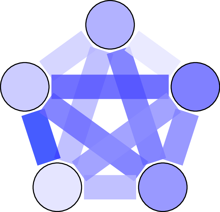
Between different pairs of parts of vertices, the density of edges could be different. For example, perhaps there are five vertex parts A, B, C, D, E; between A and B the graph looks like a random graph with edge density 0.2; between A and C the graph looks like a random graph with edge density 0.5, and so on.
An important point to emphasize is that, with a fixed error tolerance, the number of vertex parts produced by the partition does not increase with the size of the graph. This property makes the graph regularity lemma particularly useful for very large graphs.
Szemerédi’s graph regularity lemma provides us a partition of the graph that turns out to be very useful for many applications. This tool is now a central technique in modern combinatorics research.
A useful analogy is the signal-versus-noise decomposition in signal processing. The “signal” of a graph is its vertex partition together with the edge density data. The “noise” is the residual random-like placement of the edges.
Szemerédi’s idea of viewing graph theory via the lens of this decomposition has had a profound impact in mathematics. This decomposition is nowadays called “structure versus pseudorandomness” (a phrase popularized by Fields Medalist Terry Tao). It has been extended far beyond graph theory. There are now deep extensions by Fields Medalist Timothy Gowers to what is called “higher order Fourier analysis” in number theory. The regularity method has also been extended to hypergraphs.
Graph limits

László Lovász, who recently won the 2021 Abel Prize, has been developing a theory of graph limits with his collaborators over the past couple of decades. Lovász’s graph limits give us powerful tools to describe large graphs from the perspective of mathematical analysis, with applications ranging from combinatorics to probability to machine learning.
Why graph limits? Here is an analogy with our number system. Suppose our knowledge of the number line was limited to the rational numbers. We can already do a lot of mathematics with just the rational numbers. In fact, with just the language of rational numbers, we can talk about irrational numbers by expressing each irrational number as a limit of a sequence of rational numbers chosen to converge to the irrational number. This can be done but it would be cumbersome if we had to do this every time we wanted to use an irrational number. Luckily, the invention of real numbers solved this issue by filling the gaps on the real number line. In this way, the real numbers form the limits of rational numbers.
Likewise, graphs are discrete objects analogous to rational numbers. A sequence of graphs can also converge to a limiting object (what does it mean for a sequence of graphs to converge is a fascinating topic and beyond the scope of this article). These limiting objects are called “graph limits,” also known as “graphons.” Graph limits are actually simple analytic objects. They can be pictured as a grayscale image inside a square. They can also be represented as a function from the unit square to the unit interval (the word “graphon” is an amalgamation of the words “graph” and “function”). Given a sequence of graphs, we can express each graph as an adjacency matrix drawn as a black and white image of pixels. As the graphs get larger and larger, this sequence of pixel images looks closer and closer to a single image, which might be not just black and white but also could have various shades of gray. This final image is an example of a graph limit. (Actually, there are subtleties here that I am glossing over, such as permuting the ordering of the vertices before taking the limit.)
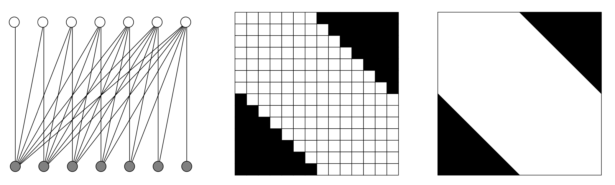
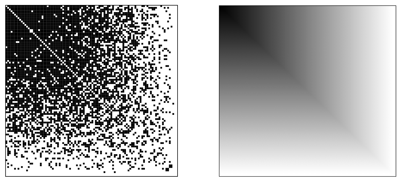
(Both images taken from Lovász’s book)
Conversely, given a graph limit, one can use it as a generative model for random graphs. Such random graphs converge to the given graph limit when the number of vertices increases. This random graph model generalizes the stochastic block model. An example of a problem in machine learning and statistics is how to recover the original graph limit given a sequence of samples from the model. There is active research work on this problem (although it is not the subject of my own research).
The mathematics underlying the theory of graph limits, notably the proof of their existence, hinges on Szemerédi’s graph regularity lemma. So these two topics are intertwined.
Sparser graphs
Graph regularity lemma and graph limits both have an important limitation: they can only handle dense graphs, namely, graphs with a quadratic number of edges, i.e., edge density bounded from below by some positive constant. This limitation affects applications in pure and applied mathematics. Real life networks are generally far from dense. So there is great interest in developing graph theory tools to better understand sparser graphs. Sparse graphs have significantly more room for variability, leading to mathematical complications.
A core theme of my research is to tackle these problems by extending mathematical tools on large graphs from the dense setting to the sparse setting. My work extends Szemerédi’s graph regularity method from dense graphs to sparser graphs. I have also developed new theories of sparse graph limits. These results illuminate the world of sparse graphs along with many of their complexities.
I have worked extensively on extending graph regularity to sparser graphs. With David Conlon and Jacob Fox, we applied new graph theoretic insights to simplify the proof of Ben Green and Terry Tao’s celebrated theorem that the prime numbers contain arbitrarily long arithmetic progressions (see exposition). It turns out that, despite being a result in number theory, a core part of its proof concerns the combinatorics of sparse graphs and hypergraphs. Our new tools allow us to count patterns in sparse graphs in a setting that is simpler than the original Green–Tao work. In a different direction, we (together additionally with Benny Sudakov) have recently developed the sparse regularity method for graphs without 4-cycles, which are necessarily sparse.
My work on sparse graph limits, together with Christian Borgs, Henry Cohn, and Jennifer Chayes , developed a new $L^p$ theory of sparse graph limits. We were motivated by sparse graph models with power law degree distributions, which are popular in network theory due to their observed prevalence in the real world. Our work builds on the ideas of Bela Bollobás and Oliver Riordan , who undertook the first systematic study of sparse graph limits. Bollobás and Riordan also posed many conjectures in their paper, but these conjectures turned out to be all false due to a counterexample we found with my PhD students Ashwin Sah, Mehtaab Sawhney, and Jonathan Tidor. These results illustrate the richness of the world of sparse graph limits.
Graph theory and additive combinatorics
A central theme of my research is that graph theory and additive combinatorics are connected via a bridge that allows many ideas and techniques to be transferred from one world to the other. Additive combinatorics is a subject that concerns problems at the intersection of combinatorics and number theory, such as Szemerédi’s theorem and the Green–Tao theorem, both of which are about finding patterns in sets of numbers.
When I started teaching as an MIT faculty, I developed a graduate-level math class titled Graph theory and additive combinatorics introducing the students to these two beautiful subjects and highlighting the themes that connect them. It gives me great pleasure to see many students in my class later producing excellent research on this topic.
In Fall 2019, I worked with MIT OpenCourseWare and filmed all my lecture videos for this class. They are now available for free on MIT OCW and YouTube. I have also made available my lecture notes, which I am currently in the process of editing into a textbook.
In my first lecture, I tell the class about the connections between graph theory and additive combinatorics as first observed by the work of Issai Schur from over a hundred years ago. Thanks to enormous research progress over the past century, we now understand a lot more, but there is still a ton of mystery that remains.
The world of large graphs is immense.
How I manage my BibTeX references, and why I prefer not initializing first names
July 4, 2021
This is both a how-to guide, and a discussion of the rationale for some of my preferences.
I use BibTeX for compiling my bibliographic references when writing math papers in LaTeX. BibTeX, when used correctly, eases the burden of bibliographic management. For example, BibTeX automatically excludes uncited references and alphabetizes the entries.
Since a single paper can have a large number of references, it is useful to have a simple system to
- Retrieve complete and accurate bibliographic records, and
- Maintain consistency.
Here are some of my own processes and conventions, along with my rationale behind some of the choices. This blog post is not a beginner’s guide on BibTeX (here is a good guide). Rather, I focus on my own conventions and choices, specifically tailored for math research papers.
Include author names as they appear in the original publication
It is common practice to shorten first names to initials in references. I do not agree with this practice. In many Asian cultures, a large fraction of the population use a fairly small number of surnames (e.g., Wang, Li, Kim). So first name initialization can lead to ambiguity. Readers are also less likely to distinguish common names and associate them with specific individuals, leading to less recognition and exposure, and this can have an adverse effect especially on early-career academics.
(Aside) As a grad student, every once in a while I was sent some combinatorics paper to referee, but these papers weren’t exactly close to anything I worked on. Looking back, I think perhaps the editors had sometimes intended to ask the other Y. Zhao in combinatorics.
(Another aside) While we are on the topic of names, it’s also worth pointing out that Chinese surnames tend to cluster late in the alphabet. This creates an interesting effect when you scroll to the bottom of a math department directory.
Economists, like mathematicians, also have co-authorship alphabetized by default. A 2006 research paper by economics professors from Stanford and Caltech showed that faculty in top 35 U.S. economics departments “with earlier surname initials are significantly more likely to receive tenure at top ten economics departments, are significantly more likely to become fellows of the Econometric Society, and, to a lesser extent, are more likely to receive the Clark Medal and the Nobel Prize,” even after controlling for “country of origin, ethnicity, religion or departmental fixed effects.” The same effects were not observed in the psychology profession, where authorship is not alphabetized.
To be clear, I am not at all advocating for abolishing the practice of ordering authors alphabetically. Quite the opposite. Ordering authors by contribution invites other conflicts and politics, which seems a lot worse. Ordering “randomly” doesn’t really make sense to me unless one can somehow enforce an independent random permutation of the authors every time the paper is read or mentioned. (End asides)
The practice of initializing first names was perhaps originally due to antiquated needs such as saving ink and space. Many journals still enforce it today in their house style.
(Example) First names are initialized not just in the references, but also sometimes in the author line, even in modern times. Up to the end of the 2006 volume, the highly regarded journal Geometric and Functional Analysis (GAFA) would typically initialize authors’ first names in the byline. There were occasional exceptions where the authors’ names were printed in full. For example, in the 2005 volume, exactly two out of 42 papers had the authors’ full names printed, and these were precisely the two papers (and only ones) having authors with Chinese names. It is likely that these authors requested to have their full names published.
When I first started writing math papers I followed what other papers did. But later on I realized that this practice does not make as much sense as I initially assumed it would. Nowadays, whenever I have control over my references (e.g., my arXiv uploads), I follow this rule:
Include author names as they appear in the original publication
Rationale and caveats:
- Why not just always use full names? Not all authors actually want their initializations expanded. Some authors may have chosen a specific stylization of their pen name (e.g., J. K. Rowling), or some specific capitalization. Also, sometimes, it is difficult to look up their full names. It is not my role to guess (just as it would never be proper for me to permute the order of authors in a paper I am citing). Following how they write their own name on their paper is the simplest and most consistent practice.
- Some authors may prefer to use different pseudonyms (or pen names) for different publications.
I should not be “correcting” them.
Some notable examples:
- Noga Alon published several papers under “A. Nilli.” Accompanying the discussion of one of such paper in Proofs from THE BOOK is a photo of a young girl with the caption “A. Nilli.”
- Victor Kac, after emmigrating from the Soviet Union, had to publish his work with his Soviet advisor Ernest Vinberg under the Italian pseudonyms Gatti and Viniberghi due to Soviet restrictions.
(I learned this fact from another fascinating economics paper on the effect of the collapse of the Soviet Union on the productivity of American mathematicians.)
Amazingly, the AMS Mathematical Reviews (MathSciNet) actually knows about author pseudonyms to high accuracy, including the examples above. There is a manual painstaking process by the Math Reviews team to assign each author to the correct person.
-
In rare instances, the publisher makes a mistake in printing the authors’ names. For example, someone told me that a journal once erroneously expanded his name as the copy editor mistakenly thought that the author’s first name was provided in a shortened form, after the final galley proof was returned to the publisher (so that there was no further opportunity for the author to correct the last minute error introduced by the copy editor). This error arose from someone deciding how someone else’s name should be written.
When there is a publication error, which name should be used in bibliographic citations? Should it matter whether or not an erratum is published? In this specific case, I would use the correct name as intended by the author, but in general, I might not have access to the extra information. These situations are annoying but rare, and can be decided case by case.
So the simplest and most consistent solution is to just include author names as they appear in the original publication.
- It is okay if some entries use full names and some others use first initials.
- It is okay if the same person appears in the references multiple times differently.
- It is not okay to change how someone’s name is intended to written.
- Initializing first names leads to ambiguity.
I admit that I have not always followed this practice, but lately I have been making an effort to do so at least when I am in charge of managing the references. The BibTeX how-to guide here makes it easy to implement. The entries imported from MathSciNet always have author names as they were originally printed.
BibTeX style file
I made a custom modification of the amsplain style file:
amsplain0.bst(click to download)
Compared to the standard amsplain style file, I made the following modifications:
- No longer displaying the MR number in the bibliographic entry;
- No longer replacing the authors by a long dash when the authors are identical to the previous entry.
To apply the new style file, I include the .bst file in the same folder as my LaTeX file, and insert the references in LaTeX using:
\bibliographystyle{amsplain0}
\bibliography{bib file name (without the .bib extension)}
Optionally, before uploading the LaTeX source to the arXiv or journal, I copy and paste the contents of the auxillary .bbl output to replace the above two lines. Then, I only have to upload a single .tex file rather than both .tex and .bbl files.
Retrieving BibTeX entries from MathSciNet
For the most part, you do not need to enter BibTeX entries by hand. MathSciNet has already compiled all this information.
- Accessing MathSciNet requires a subscription, which many universities have. Common ways to access MathSciNet:
- From a device on campus network;
- Using university VPN;
- Using university library’s proxy url;
- Using AMS Remote access to first pair your browser with AMS when you’re on campus or on VPN, so that you can continue accessing MathSciNet and other AMS resources later even when off-campus and off-VPN.
- You can configure your browser to search for MathSciNet directly from the search bar. For example, in Chrome, in Settings / Search Engine you can add a new search engine with the following configurations
- Search engine: MR search by title
- Keyword:
mr - Query url:
https://mathscinet.ams.org/mathscinet/search/publications.html?pg1=TI&s1=%s&extend=1
to search MathSciNet by title. For instance, typing
mr large graphinto the search bar yields a search for articles with both words “large” and “graph” in the title, whereas typingmr "large graph"into the search bar yields a search for papers with the phrase “large graph” in the title. You can also configure other custom searches by modifying the query url. - A free lite version, MR Lookup, can be used without subscription, though it only displays the top three search results. It also gives the results in BibTeX format.
All articles listed on MathSciNet can be extracted as BibTeX entries, either individually or in bulk (this can be done on the MathSciNet website by selecting BibTeX from the drop down menu).
-
I like using BibDesk (only on Mac; free and comes with TeXShop), which offers a nice interface for BibTeX management, including automatic import from MathSciNet (from the External–Web tab on the left). BibDesk also has other useful automated tools such as batch renaming entry keys according to authors-year. (Update: BibDesk is not currently compatible with the updated interface of MathSciNet. You can get around this issue by using the older version of MathSciNet.)
I imagine there must be other similar BibTeX management tools with automatic MathSciNet import, but I have not personally used any of them. See this discussion.
Most entries from MathSciNet are accurate and consistently formatted, especially for published journal articles. MathSciNet has a dedicated staff for maintaining the quality of its entries. They follow the official AMS journal title abbreviations (best not to make up these abbreviations yourself). In contrast, other sources (e.g., Google Scholar search) often produce inconsistently formatted and inaccurate bibliographic entries.
Manual additions and edits
Occasionally some entries need to be added or edited by hand. Here are some common scenarios in my experience.
Additions:
- Pre-print and pre-published articles (including those appearing first on the publisher website but not yet assigned an issue) do not appear in MathSciNet. I add them manually as follows:
- For arXiv preprints:
@misc{Smi-ar, AUTHOR = {John Smith}, TITLE = {I proved a theorem}, NOTE = {arXiv:2999.9999}, } - For papers to appear (use official AMS journal title abbreviations)
@article{Smi-mj,
    AUTHOR  = {John Smith},
    TITLE   = {I proved an excellent theorem},
    JOURNAL = {Math. J.},
    NOTE    = {to appear},
}
(It might annoy some people to have an @article entry without a year, but shrug, it compiles, and I haven’t found a more satisfactory solution.)
- For arXiv preprints:
- Really old (like, pre-1940) and some foreign language articles/books are not listed on MathSciNet — I copy the citations from somewhere else and enter them as an @article/@book by hand.
- For non-standard entries like websites and blog posts, I add them as @misc similar to arXiv entries, using the
notefield as a catch-all. (Yes I know that there is specifically a @url entry type, but I find it easier and more predictable to use @misc. In any case, the choice of entry type does not show up in the output.) - Capitalizations.
By default, BibTeX changes the entire title to lower case except for the very first letter. To keep capitalizations of proper nouns, LaTeX commands, etc., surround those letters/words by
{...}. BibTeX entries from MathSciNet usually gets this right automatically, but more care if needed when manually adding entries such as from the arXiv.
Modifications:
- MathSciNet usually gets it right but sometimes accented names need some manual editing to compile correctly. A notable exaple is that when “Erdős” appears in a title, one needs to surround the ő
\H{o}by{...}, e.g.,{E}rd{\H{o}}, or else BibTeX changes\Hto\hthereby causing a compilation error. Similar issues also arise in the author field, e.g., with the Polish Ł\L. They can always be fixed by surrouding the problematic snippets by{...}. - Some MathSciNet entries for books have extraneous data that should be deleted. It is usually clear what’s going on after seeing the output PDF.
- For some journals with reboots in its publication history, the official AMS journal title abbreviation sometimes includes a “series” number, e.g., Annals of Mathematics is actually Annals of Mathematics. Second Series abbreviated as Ann. of Math. (2), which is consistent with MathSciNet imports. Some people don’t like to keep the (2). I’m okay either way.
- Conference proceedings are the worst offenders on consistent formatting. They are not covered by AMS guidance and it is a free-for-all. Basically, I import from MathSciNet, compile and see what the PDF output looks like, and then delete extraneous data. If a conference proceeding article is superseded by a journal article, I use the journal article instead.
- MathSciNet BibTeX entries include a bunch of other extraneous information like the reviewer’s name. I could delete them but these do not show up in the output anyway, so I don’t bother. The only piece that does show up in the amsplain style is MR number, which does not show up in my modified amsplain0 style.
Entry keys
The simplest cases:
- Single author: the first up to three letters of surname (preserving capitalization), followed by two-digit year. Example:
Wil95in@article {Wil95, AUTHOR = {Wiles, Andrew}, TITLE = {Modular elliptic curves and {F}ermat's last theorem}, JOURNAL = {Ann. of Math.}, VOLUME = {141}, YEAR = {1995}, NUMBER = {3}, PAGES = {443--551}, } - Multiple authors: a string of initialized surnames followed by two-digit year. Example:
ER60in@article {ER60, AUTHOR = {Erd\H{o}s, P. and R\'{e}nyi, A.}, TITLE = {On the evolution of random graphs}, JOURNAL = {Magyar Tud. Akad. Mat. Kutat\'{o} Int. K\"{o}zl.}, VOLUME = {5}, YEAR = {1960}, PAGES = {17--61}, }
In BibDesk, I automatically assign keys via the following configuation: in BibDesk Preferences / Cite Key Format, select
- Present Format: Custom
- Format String:
%a91%y%u0
Select one or more rows/entries, enter Cmd-K to automatically generate keys. For multi-author entries, this correctly generates the key, e.g., ER60 (unless there are more than nine authors). For single-author entries, a bit of manual work is needed to change from W95 to Wil95 (I prefer not leaving it like W95 since it leads to more conflicts and confusion).
Where it gets a bit more tricky:
- If the above rules produce conflicting keys:
- Add a suffix to the key with a few letters containing some informative data such as journal name or topic, e.g.,
[Wil95ann],[ER60rg], or - Distinguish the keys by letters, e.g.,
[Wil95a][Wil95b](this is what BibDesk does automatically; but this system could potentially be more confusing later on).
- Add a suffix to the key with a few letters containing some informative data such as journal name or topic, e.g.,
- Pre-prints or pre-publications:
- Forget the year, e.g.,
[XYZ], and if disambiguation is needed, add a dash followed by some informative letters, e.g.,[XYZ-gcd]
- Forget the year, e.g.,
- Not sure which year to use? E.g., a proceeding published in 2000 for a conference held in 1999. Use the
yearfield in BibTeX as imported by MathSciNet.
What the BibTeX output looks like
Using the amsplain0 style file from the beginning, a citation \cite{Wil95} produces
References
[1] Andrew Wiles, Modular elliptic curves and Fermat’s last theorem, Ann. of Math. 141 (1995), 443–551.
And that’s it! This is how I manage my BibTeX.
The cylindrical width of transitive sets
January 28, 2021
The high dimensional sphere comes many surprising and counterintuitive features. Here is one of them.
We say that a subset $X$ of the unit sphere in $\mathbb{R}^d$ is transitive if, informally, one cannot distinguish one point of $X$ from another if we are allowed to rotate/reflect. Formally, we say that $X$ is transitive if the group of isometries of $X$ acts transitively on it. This is equivalent to saying that $X$ is the orbit of some point under the action of some subgroup of the orthogonal group.
Perhaps you, like me, can only visualize in three-dimensions. Here are some examples:
- Every regular polytope (platonic solid) is transitive.
- Start with an arbitrary vector, and consider all points obtained by permuting its coordinates, as well as switching the signs of some of the coordinates. The resulting set is transitive (this is a generalization of the permutahedron.) A specific example is given below.
- The whole sphere itself is transitive
The finite examples look like they can be fairly spread out on the sphere. However, this intuition turns out to be completely wrong in high dimensions. All finite transitive sets in high dimensions have small width, meaning that they lie close to some hyperplane (in sharp contrast to the whole unit sphere, which has width 2).
I had conjectured the following statement, which was proved by Ben Green.
Theorem (Green). Every finite transitive set of unit vectors in $\mathbb{R}^d$ lies within distance $O\bigl(\frac{1}{\sqrt{\log d}}\bigr)$ of some hyperplane.
This bound is actually tight for the example obtained by taking all signings and permutations of the unit vectors
\[\frac{1}{\sqrt{H_d}}\Biggl(\pm 1, \frac{\pm 1}{\sqrt{2}}, \frac{\pm 1}{\sqrt{3}}, \ldots, \frac{\pm 1}{\sqrt{d}}\Biggr)\]where
\[H_d = 1 + \frac{1}{2} + \cdots + \frac{1}{d} \sim \log d.\]Green’s proof, among other things, uses the classification of finite simple groups.
Our new results: finite transitive sets have small cylindrical width
In our new paper, The cylindrical width of transitive sets, coauthored with Ashwin Sah and Mehtaab Sawhney, we generalize Green’s result to show that not only do transitive sets lie close to a hyperplane, but they also lie close to some codimension-$k$ subspace for every $k$ that is not too large.
Theorem (Sah–Sawhney–Zhao). There exists some constant $C$ so that for every $1 \le k \le d/(\log d)^C$, every finite transitive set of unit vectors in $\mathbb{R}^d$ lies within distance $O\bigl(\frac{1}{\sqrt{\log (d/k)}}\bigr)$ of codimension-$k$ subspace.
The bound $O\bigl(\frac{1}{\sqrt{\log (d/k)}}\bigr)$ is tight up to a constant factor. We conjecture that the hypothesis $1 \le k \le d/(\log d)^C$ can be removed:
Conjecture. For every $1 \le k \le d$, every finite transitive set of unit vectors in $\mathbb{R}^d$ lies within distance $O\bigl(\frac{1}{\sqrt{\log (2d/k)}}\bigr)$ of codimension-$k$ subspace.
Finally, we conjecture that not only do finite transitive sets lie close to subspaces, but they can be completely contained in a small cube. All examples known to us are consistent with this conjecture, even though I still find it very counterintuitive.
Conjecture (Finite transitive sets lie in a small cube). Every finite transitive set of unit vectors in $\mathbb{R}^d$ is contained in a cube of width $O\bigl(\frac{1}{\sqrt{\log d}}\bigr)$.
Even proving a bound of $o(1)$ (as $d\to \infty$) would be quite interesting.
Both conjectures are generalizations of Green’s result, but the relationship between the two conjectures is unclear.
Ashwin Sah and Mehtaab Sawhney win the Morgan Prize
October 29, 2020
Congratulations to Ashwin Sah and Mehtaab Sawhney for winning the 2021 AMS-MAA-SIAM Frank and Brennie Morgan Prize for Outstanding Research in Mathematics by an Undergraduate Student! This is the most prestigious prize in the US for undergraduate mathematics research (though I must say that their work far surpasses that of “undergraduate research”). It is also the first time in the history of the Morgan Prize for it to be jointly awarded to more than one recipient.
From the prize citation:
The award recognizes the duo’s innovative results across a broad range of topics in combinatorics, discrete geometry, and probability.
The prize committee notes, “Working alongside one another, Sah and Sawhney settled longstanding conjectures and improved results by established mathematicians. The research of Sah and Sawhney is both deep and broad, tackling questions at the very forefront of current research, yet extending across the entire gamut of modern combinatorics, with significant contributions to extremal graph theory, graph limits, additive combinatorics, Ramsey theory, algebraic combinatorics, combinatorial geometry, random graphs and random matrix theory. They have demonstrated a significant amount of ingenuity, originality and technical ability, resulting in a research record, which is extremely rare for undergraduate students.”
Combined, Sah and Sawhney have authored 30 papers (11 together), and published in top journals, including Inventiones Mathematicae, Advances in Mathematics, Mathematical Proceedings of the Cambridge Philosophical Society, the Journal of Combinatorial Theory Series B, and Combinatorica.
(The paper count in the award citation was taken from earlier this year and is now already quite a bit out of date.)
I got to know both Ashwin and Mehtaab as students in my Putnam Seminar and graduate combinatorics class during their very first undergraduate semester at MIT. Since then, they have led an intensively productive and ongoing collaboration, producing an incredible amount of fantastic research results across a wide spectrum of topics in combinatorics, probability, number theory, and algorithms. It was a great pleasure for me to be working with Ashwin and Mehtaab on many of these projects. Some of their work were previously featured on this blog:
- The number of independents in an irregular graph
- A reverse Sidorenko inequality
- New upper bounds on diagonal Ramsey numbers
- Singularity of discrete random matrices
Ashwin and Mehtaab are now both first-year PhD students at MIT. I’m sure that we will see a lot more coming from them.
Jain–Sah–Sawhney: Singularity of discrete random matrices
October 13, 2020
Vishesh Jain, Ashwin Sah, and Mehtaab Sawhney just posted two amazing papers: Singularity of discrete random matrices Part I and Part II.

The singularity problem for random matrices: what is the probability that a random $n\times n$ matrix with independent 0/1 entries is singular?
The first non-trivial bound on this problem was by Komlós in 1967. After a long series of works by many mathematicians including Kahn, Komlós, Szemerédi, Tao, Vu, Bourgain, Wood, Rudelson, and Vershynin, a breakthrough was recently achieved by Tikhomirov, who showed that, when the matrix entries are iid uniform from \(\{0,1\}\), the probability of singularity if $(1/2 + o(1))^n$, which is tight since with probability $2^{-n}$ the first row is zero.
The new papers of Jain–Sah–Sawhney consider a natural extension of the singularity problem where each entry of the $n\times n$ matrix is iid: 1 with probability $p$ and 0 with probability $1-p$, for some value of $p$ other than 1/2.
A folklore conjecture in this area states that the main reason for the singularity of such random matrices is the presence of two equal rows/columns or some zero row/column:
Conjecture. For a fixed $0 < p < 1$, the probability that a random $n\times n$ matrix with iid Bernoulli(p) entries is singular is $1+o(1)$ times the probability that the matrix has one of the following: (a) two equal rows, (b) two equal columns, (c) a zero row, (d) a zero column.
Note that even Tikhomirov’s breakthrough result does not give precise enough results to answer this conjecture. However, we now have the following incredible result.
Theorem. (Jain–Sah–Sawhney) The above conjecture is true for all $p \ne 1/2$.
(The case $p = 1/2$ remains open.)
In fact, they prove something much more general: namely that the above result remains true if the random matrix entries are iid discrete random variables that are non-uniform on its support. Furthermore, they prove nearly tight bounds on the probability of these matrices having small least singular values. Very impressive!
Gunby: Upper tails for random regular graphs
October 5, 2020
Ben Gunby, a final-year PhD student at Harvard whom I advise, just posted his paper Upper tails of subgraph counts in sparse regular graphs. This is a substantial paper that unveils surprising new phenomena for the problem of large deviations in random graphs.
Problem. What is the probability that a random graph has far more copies of some given subgraph than expected?
This is called the “upper tail” problem for random graphs. It is a problem of central interest in probabilistic combinatorics. There was a lot of work on this problem for the classic Erdős–Rényi random graph $G(n,p)$ (with edges appearing independently at random), with a lot of exciting recent developments. Ben considers the upper tail problem for random regular graphs, another natural random graph model. Random regular graphs are usually harder to analyze since the random edge appearance are no longer independent, and this increased difficulty also shows up for the upper tail problem.
Let me highlight one specific result in Ben’s paper (Theorem 2.9).
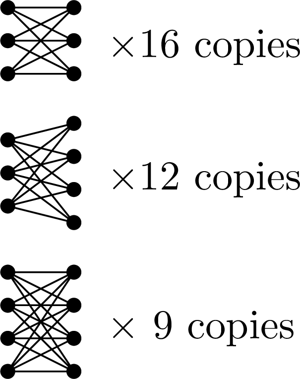
Theorem. (Gunby) Let \(G_n^d\) be a random $n$-vertex $d$-regular graph, where $d = d(n)$ depends on $n$. Assume that $dn$ is even and and \(n^{14/15}\log n \le d = o(n)\). Let $X$ denote the number of copies of
 in \(G_n^d\). Then for every fixed \(\delta > 0\) (here \(\sim\) means up to $1+o(1)$ factor),
This result is surprising. The appearance of the fractional power of the log factor has not been observed in previous works on the upper tail problem. It is even more impressive that Ben was able to prove such a sharp estimate.
Understanding these large deviation probabilities roughly corresponds to understanding the “dominant reason” for rare events. Roughly speaking, the fractional power of log appears because the dominant reason is not the presence of some fixed subgraph (e.g., a large clique or hub), unlike all earlier results, which have asymptotics of the form \(n^2 p^d \log(1/p)\). Something else more subtle is happening. While we still do not understand the complete picture, Ben’s result provides strong evidence why the upper tail problem for random regular graphs may be substantially more intricate than that of $G(n,p)$.
In this blog post, I will tell you some history and background of the upper tail problem in random graphs. I will try to explain why Ben’s result is surprising. Lastly, I will also mention a recent paper I have with Yang Liu on the upper tail problem in random hypergraphs, where a different new phenomenon is observed.
Chasing the infamous upper tail
Roughly, and intuitively, to gain a precise understanding of the upper tail problem, we are really asking:
What are the dominant reasons for the rare event that a random graph $G(n,p)$ has way too many triangles?
We can now say confidently the following:
It is primarily because the such a rare random graph contains roughly a large clique or a large hub.
Here a “hub” is a set of vertices adjacent to all other vertices. It is not hard to see that planting a large clique or hub in a $G(n,p)$ would automatically generate many additional triangles (these triangles may use also the edges of the random graph).
For example, the following theorem is the culmination of a long line of work by many researchers.
(We use the following asymptotic notation, which is standard in this line of work: \(f \ll g\) means $f = o(g)$.)
Theorem. Let $X$ denote the number of triangles in $G(n,p)$. Then, for $n^{-1/2} \ll p \ll 1$ and fixed $\delta > 0$, one has
\[-\log \mathrm{Pr}(X \ge (1+\delta) \mathbb{E} X) \sim \min \left\{\frac{\delta}{3}, \frac{\delta^{2/3}}{2}\right\} n^2p^2\log\frac{1}{p}\]The problem of estimating the upper tail $\mathrm{Pr}(X \ge (1+\delta) \mathbb{E})$ has a long history. Janson and Rucinski called this problem the infamous upper tail, which had resisted a wide range of techniques that researchers have used to tackle this problem. This upper tail problem was an excellent litmus test in the development of concentration inequalities.

Several significant breakthroughs then occurred on this problem over the past decade.
DeMarco–Kahn and Chatterjee independently determined the order of magnitude of the log-probability in the above upper tail problem, for triangle counts in a random graph. Their work closed a log-factor gap left by previous methods developed by Kim–Vu.
The next goal was then to pinpoint the tail probability. This led to further developments of powerful tools.
The seminal work of Chatterjee and Varadhan developed a large deviation principle for the upper tail problem in random graphs, thereby reducing the problem to a variational problem in the space of graphons, i.e., graph limits. Their work paved the way for much further development, which has two complementary strands:
1. Extending the large deviation framework to sparser graphs. Chatterjee and Varadhan’s proof uses Szemerédi’s graph regularity lemma, which only allows us to handle dense graphs (here for random graphs $G(n,p)$ dense means constant $p$, whereas sparse means $p = o(1)$). Further work, starting with Chatterjee–Dembo’s “non-linear large deviations”, as well as further improvements by Eldan, Cook–Dembo, Augeri, Harel–Mousset–Samotij, and Basak–Basu, allow us to handle much sparser densities of graphs.
For certain subgraphs, including cliques, we now have a very precise understanding thanks to Harel–Mousset–Samotij, who gave a short and clever container-inspired combinatorial argument in the case of triangles.
2. Solving the variational problem. The above large deviation frameworks reduces the problem of estimating the tail probability to another problem—a variational problem in the space of graphons.
Variational problem for upper tails: Among edge-weighted graphs with some prescribed subgraph density, determine the minimum possible relative entropy (a certain non-linear function of the edge-weights)
These variational problems are more difficult than classical problems in extremal graph theory. In fact, despite some progress, we still do not understand how to solve such problems exactly in the “dense” regime.
For sparse graphs $G(n,p)$ with $p \to 0$, the variational problem was solved asymptotically in the case of clique subgraphs by Lubetzky–Zhao, and for more general subgraph counts by Bhattacharya–Ganguly–Lubetzky–Zhao.
The two complementary strands together pinpoint upper tail probabilities. Similar to the case of triangles, the main message is, roughly speaking,
The dominant reason for a random graph to have too many copies of some fixed $H$ is that it contains a large clique or a large hub.
Theorem. Let $H$ be a graph with maximum degree \(\Delta\). Let $\delta > 0$. Let $X$ be the number of copies of $H$ in $G(n,p)$. Provided that $n^{-\alpha_H} \le p = o(1)$ (where $\alpha_H$ is some explicit constant that has improved over time), one has
\[-\log \mathrm{Pr} (X \ge (1+\delta)\mathbb{E} X) \sim c(H, \delta) p^{\Delta} n^2 \log \frac{1}{p},\]where \(c(H,\delta) > 0\) is an explicit constant determined in Bhattacharya–Ganguly–Lubetzky–Zhao.
While this is a pretty satisfactory formula, our understanding is still not complete.
-
Is the result valid for the “full” range of $p$?
-
What precise statements can you make about the conditioned random graph? (see Harel–Mousset–Samotij)
Gunby’s work on random regular graphs
Ben Gunby’s work studies the upper tail problem for random regular graphs:
Problem. Let $X$ be the number of copies of some given subgraph $H$ in a random $d$-regular graph $G_n^d$. Estimate $-\log \mathrm{Pr}(X \ge (1+\delta)\mathbb{E} X)$, when \(n^{1-c} \le d = o(n)\).
There is a similar dichotomy of steps as above:
-
Proving a large deviations framework. The upper bound to the probability can be deduced from the corresponding theorems for $G(n,p)$, while the lower bound requires new and lengthy arguments.
-
Solving the variational problem – this is where new difficulties and innovations lie.
A recent paper of Bhattacharya–Dembo (this is by Sohom Bhattacharya and not my coauthor Bhaswar Bhattacharya mentioned earlier) essentially solved the variational problem when $H$ is a regular graph (Ben had also independently worked out the case when $H$ is a cycle).
Ben Gunby’s new paper solves the variational problem for “most” graphs $H$ (those that satisfy some technical condition), which includes all graph $H$ with average degree greater than 4, as well as pretty much all small graphs.
For most graphs $H$, the upper tail has “expected” behavior, meaning that the dominant reason for seeing many copies of $H$ is, very roughly speaking, the presence of some large planted subgraph. The resulting tail probability formulas also resemble what we have seen earlier:
\[-\log \mathrm{Pr}(X \ge (1+\delta) \mathbb{E} X) \sim \rho(H, \delta) n^2 (d/n)^{2+\gamma(H)} \log(n/d).\]for some graph parameter \(\gamma(H)\), whose role here is far from obvious.
For every graph $H$, Ben manages to bound the log-probablity within a log-factor gap:
\[n^2 (d/n)^{2+\gamma(H)} \lesssim -\log \mathrm{Pr}(X \ge (1+\delta) \mathbb{E} X) \lesssim n^2 (d/n)^{2+\gamma(H)} \log(n/d)\]The most surprising part of Ben’s paper is that for some $H$, the upper tail is not “expected” as above, i.e., the asymptotic formula two display equations earlier is incorrect for this $H$.
For the graph , Ben solves the variational problem, which led to the formula at the beginning of this post. The solution turns out to come not from “planting a subgraph” but rather from some other more delicate construction.
It remains to be seen what happens to other graphs $H$. Will we need even more intricate constructions? What does this mean for techniques towards solving the upper tail problem for the full range of degree parameters? There is still lot that we do not understand.
Large deviations for random hypergraphs
In a recent paper with Yang Liu (to appear in Random Structures & Algorithms), we considered the extension of the upper tail problem to random hypergraphs. Yang Liu is a PhD student at Stanford. We started this work while Yang was an undergraduate student at MIT.

Consider the random $k$-uniform hypergraph \(G^{(k)}(n,p)\), where every unordered $k$-tuple of vertices appears as an edge independently with probability $p$.
Problem. Given a $k$-uniform hypergraph $H$. Let $X$ denote the number of copies of $X$ in \(G^{(k)}(n,p)\). Estimate $\mathrm{Pr}(X \ge (1+\delta)\mathbb{E} X)$.
As before, there are two complementary strands (1) developing large deviation framework and (2) solving the variational problem. Some of the work towards (1) for random graphs can be transferred over to the hypergraph setting. Towards (2), we solve the variational problem asymptotically for some $H$, and make a conjecture for what we believe should happen for general $H$.
We show that one cannot naively extend the upper tail results from random graphs to random hypergraphs. In our paper, we take the readers on a long discussion through several iterations of naive conjectures and counterexamples, eventually building up to our final conjecture, which takes some effort to state, but very roughly, says that
The dominant reason for upper tails in random hypergraphs is the presence of a collection of “stable mixed hubs.”
For both random regular graphs and random hypergraphs, these recent results highlight unexpected phenomena. They illustrate the richness of the problem and lead us to more questions than answers.
Joints of varieties
September 12, 2020
The summer has come to an end. The temperature in Boston seems to have dropped all the sudden. Our fall semester has just started, though without all the new and returning students roaming around campus this time (most classes are online this term). I quite miss the view from my MIT office, and all the wonderful people that I would run into the department corridors.

I’ve been working from home for the past several months and connecting with my students via Zoom. In this and the upcoming several posts, I would like to tell you about some of the things that we have been working on recently.
With PhD student Jonathan Tidor and undergraduate student Hung-Hsun Hans Yu, we recently solved the joints problem for varieties by a developing a new extension of the polynomial method. (Also see my talk video and slides on this work.)

I discussed the joints problem in an earlier blog post. Recall that the joints problem asks:
Joints problem: At most how many joints can $N$ lines in $\mathbb{R}^3$ can make?
Here a joint is a point contained in three non-coplanar lines.
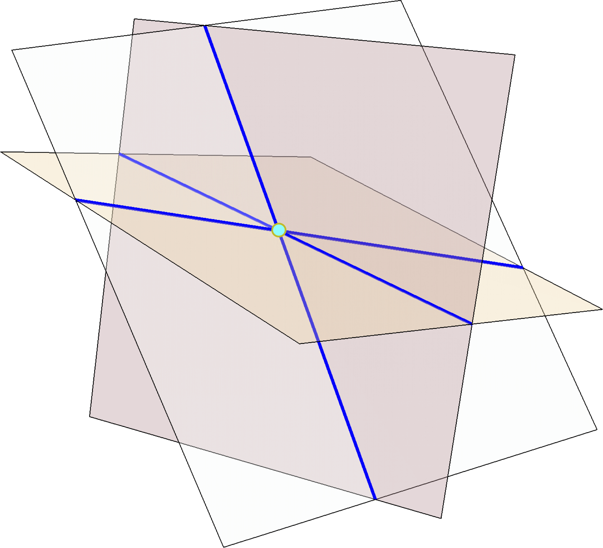
Here is an example of a configuration of lines making many joints. Take k generic planes in space, pairwise intersect them to form \(N = \binom{k}{2}\) lines, and triplewise intersect to form \(J = \binom{k}{3} \sim \frac{\sqrt{2}}{3} N^{3/2}\) joints.
The joints problem was raised in the early 1990’s. It is a problem in incidence geometry, which concerns possible incidence patterns of objects like points and lines. The joints problem has also received attention from harmonic analysts due to its connections to the Kakeya problem.
The big breakthrough on the joints problem was due to Guth and Katz, who showed that the above example is optimal up to a constant factor:
Joints theorem (Guth–Katz). $N$ lines in \(\mathbb{R}^3\) form $O(N^{3/2})$ joints.
Guth and Katz solved the problem using a clever technique known as the polynomial method, which was further developed in their subsequent breakthrough on the Erdős distinct distances problem. The polynomial method has since then grown into a powerful and indispensible tool in incidence geometry, and it also led to important recent developments in harmonic analysis.
I learned much of what I know about the polynomial method from taking a course by Larry Guth while I was a graduate student. Guth later developed the course notes into a beautifully written textbook, which I highly recommend. A feature of the expository style of this book, which I wish more authors would adopt, is that it frequently motivates ideas by first explaining false leads and wrong paths. As I was reading this book, I felt like that I was being taken on a journey as a travel companion and given a lens towards the thinking process, rather than somehow being magically teleported to the destination.
In my previous paper on the joints problem with Hans Yu, which I discussed in earlier blog post, we sharpened the Guth–Katz theorem to the optimal constant.
Theorem (Yu–Zhao). $N$ lines in \(\mathbb{R}^3\) have \(\le \frac{\sqrt{2}}{3} N^{3/2}\) joints.
Everything I have said so far are also true in arbitrary dimensions and over arbitrary fields, but I am only stating them in \(\mathbb{R}^3\) here to keep things simple and concrete.
Joints of flats
Our new work solves the following extension of the joints problem.
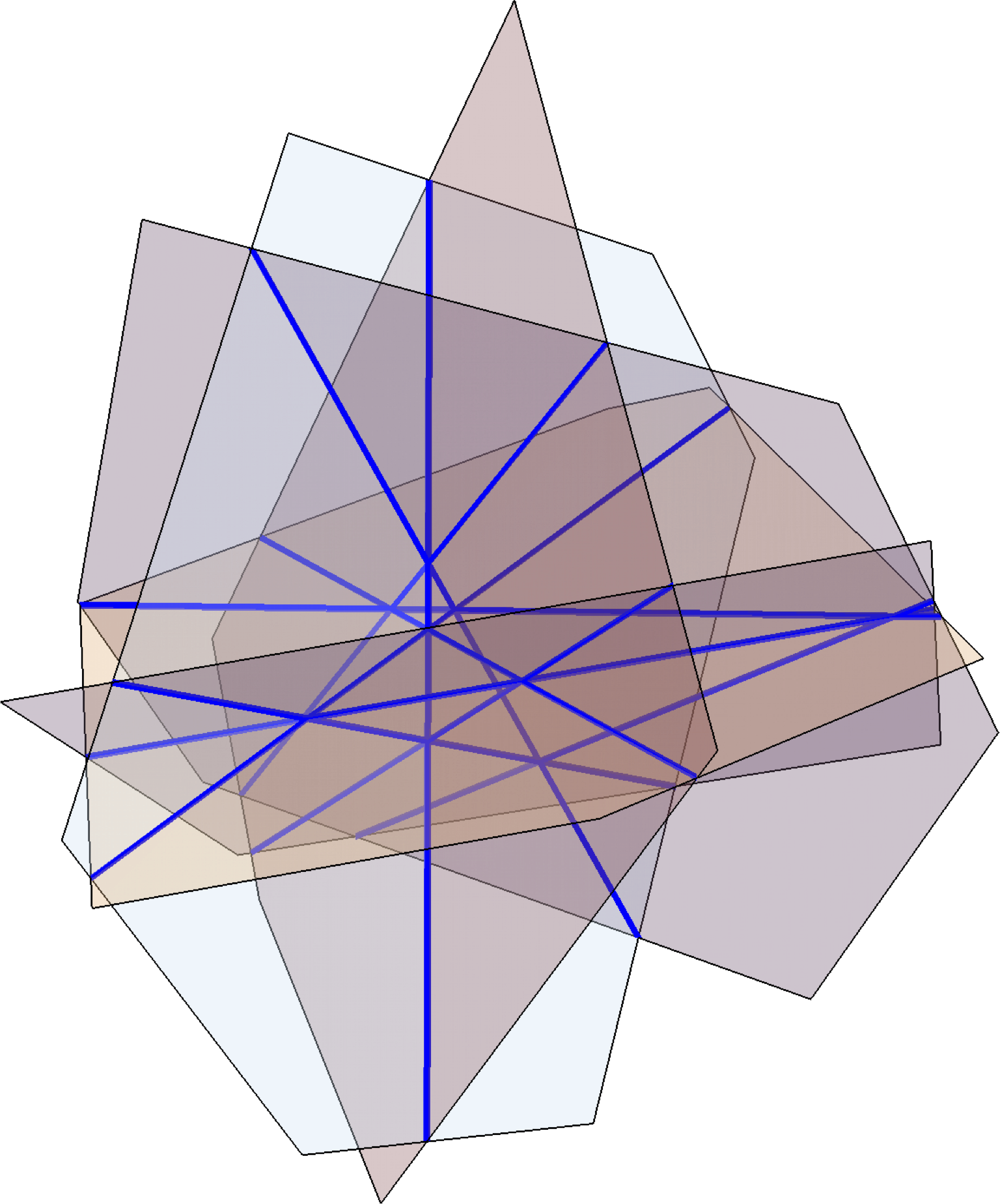
Joints problem for planes. At most how many joints can $N$ planes in \(\mathbb{R}^6\) make?
Here a joint is a point contained in a triple of 2-dimensional planes not all contained in some hyperplane.
The example given earlier for joints of lines extends easily to joints of planes.
Example. Take $k$ generic 4-flats in \(\mathbb{R}^6\), pairwise intersect them to form $N = \binom{k}{2}$ planes, and triplewise intersect them to form \(\binom{k}{3} = \Theta(N^{3/2})\) joints.
Joints of planes concerns incidences between high dimensional objects, which in general tend to be more intricate compared to incidence problems about points and lines.
I first learned about this problem from a paper of Ben Yang, who did this work as a PhD student of Larry Guth. Yang proved that $N$ planes in \(\mathbb{R}^6\) form at most $N^{3/2+o(1)}$ joints. His proof uses several important recent developments in incidence geometry, and in particular uses the polynomial partitioning technique of Guth and Katz (as well as subsequent extensions due to Solymosi–Tao and Guth). This is a fantastic result, though with two important limitations due to the nature of the method:
- There is an error term in the exponent $N^{3/2+o(1)}$ that is conjectured not to be there. One would like a bound of the form $O(N^{3/2})$
- The result is restricted to planes in \(\mathbb{R}^6\) and does not work if we replace \(\mathbb{R}\) by an arbitrary field. This is because the polynomial partitioning method uses topological tools, in particular the ham sandwich theorem, which crucially requires the topology of the reals.
Our work overcomes both difficulties. As a special case, we prove (here \(\mathbb{F}\) stands for an arbitrary field, and the hidden constants do not depend on \(\mathbb{F}\)):
Joints of planes (Tidor–Yu–Zhao). $N$ planes in \(\mathbb{F}^6\) have $O(N^{3/2})$ joints.
And more generally, our results hold for varieties instead of flats. Here a joint is a point contained in a triple of varieties, such that it is a regular point on each of the three varieties and the three tangent plane do not lie inside a common hyperplane.
Joints of varieties (Tidor–Yu–Zhao). A set of 2-dimensional varieties in \(\mathbb{F}^6\) of total degree $N$ has $O(N^{3/2})$ joints.
The above statements are special cases of our results. The joints problem for lines is known to hold under various extensions (arbitrary dimension and fields, several sets/multijoints, counting joints with multiplicities), and our theorem holds in these generalities as well.
Proof sketch of the joints theorem for lines
Here is a sketch of the proof that $N$ lines in \(\mathbb{R}^3\) make $O(N^{3/2})$ joints (following the simplifications due to Kaplan–Sharir–Shustin and Quilodrán; also see Guth’s notes for details of the proof).
The first two steps below are both hallmarks of the polynomial method, and they are present in nearly every application of the method. The third step is a more joints-specific argument.
-
Parameter counting. The dimension of the vector space of polynomials in \(\mathbb{R}[x,y,z]\) up to degree $n$ is \(\binom{n+3}{3}\). We deduce that if there are $J$ joints and \(J < \binom{n+3}{3}\), then one can find a nonzero polynomial $g$ of degree $\le C J^{1/3}$ (for some constant $C$) that vanishes on all the joints (as there are more coefficients to choose from than there are linear constraints). Take such a polynomial $g$ with the minimum possible degree.
-
Vanishing lemma. A nonzero single variable polynomial cannot vanish more times than its degree.
-
If all lines have $> CJ^{1/3}$ joints, then the vanishing lemma implies that $g$ vanishes on all the lines. At each joint, $g$ vanishes identically along three independent lines, and hence its directional derivatives vanish in three independent directions, and thus the gradient \(\nabla g\) vanishes at the joint. Therefore, the three partial derivatives \(\partial_x g\), \(\partial_y g\), \(\partial_z g\) all vanish at every joint, and at least one of them is a nonzero polynomial and has smaller degree than $g$, thereby contradicting the minimality of the degree of $g$. Therefore, the initial assumption must be false, namely that some line has \(\le C J^{1/3}\) joints. We can then remove this line, deleting \(\le CJ^{1/3}\) joints, and proceed by induction to prove that $J = O(N^{3/2})$.
Some wishful thinking
It is natural to try to extend the above proof for the joints problem for planes. One quickly runs into the following conundrum:
How does one generalize the vanishing lemma to 2-variable polynomials?
The vanishing lemma is such an elementary fact about how polynomial behaves on a line. Yet it plays a crucial role in the polynomial method. We would be able to adapt the above proof to joints of planes if only something like the following would be true (they are not):
Wishful thinking 1. Show that every nonzero polynomial $g(x,y)$ of degree $n$ has $O(n^2)$ zeros.
Well, this is obviously nonsense. The zero set of $g(x,y)$ is typically a curve with infinitely many points.
How else might we try to extend the vanishing lemma to two dimensions? Bézout’s theorem is one such extension. It tells us that two polynomials $g(x,y)$ and $h(x,y)$ without common factors cannot have more than $(\deg g)(\deg h)$. So, perhaps, instead of trying to find one polynomial vanishing at all joints, we try to find a pair of polynomials.
Wishing thinking 2. Show that one can find two polynomials \(g, h \in \mathbb{R}[x_1, x_2, x_3, x_4, x_5, x_6]\) vanishing at all $J$ joints and $(\deg g)(\deg h) = O(J^{1/3})$, and such that $g$ and $h$ have no common factors when restricted to any of the given planes.
This approach is a natural one to try for the joints of planes problem, and is an approach that many people have thought about. It also seems extremely hard to get it to work (likely impossible). It seems closely related to the inverse Bézout problem, which already illustrates some of the difficulties encountered.
Instead of asking a polynomial to vanish at every joint, we can demand more. Namely that we can ask the polynomial to vanish at each joint to some high order (equivalently, asking some derivatives of the polynomial to vanish at the joints). This idea (sometimes called the “method of multiplicities”) has shown to be useful in a variety of contexts. Perhaps we can modify Wishing thinking 1 to account for these multiplicities?
Wishful thinking 3. Show that every nonzero polynomial $g(x,y)$ of degree $n$ can vanish to order $s$ at no more than $O(n^2/s^2)$ points.
The reason why one might hope for such a statement is that there are \(\binom{n+2}{2} \approx n^2/2\) degrees of freedom for choosing $g$, and this number is roughly the same as the number of constraints associated to forcing the polynomial to vanish to order $s$ at $n^2/s^2$ points.
However, Wishful thinking 3 is still too good to be true. For example, the polynomial $g(x,y) = y^s$ is a low-degree polynomial that vanishes to order $s$ at every point on the $x$-axis.
So what was wrong with the parameter counting intuition? It must be the case that some of the linear constraints associated to these high order vanishing constraints are linearly dependent.
Extending the polynomial method
So far all I have told you are what doesn’t work, and I haven’t said anything about what does work. Where we left off above is a good starting point of what we actually do, which I will not describe here in this blog post but instead refer you to either my talk or our paper for details. We have to account for the linear dependencies between these higher order vanishing conditions, and we come up with a process of assigning non-redundant vanishing conditions (each in the form of some higher order derivative operator evaluated at a joint). We prove a new vanishing lemma tailored for this joints problem. Rather vaguely, it has the following form:
A new vanishing lemma. Given a finite set of planes in \(\mathbb{R}^6\) forming some joints, and a positive integer $n$, and an integer (“handicap”) attached to each joint, we run a certain process that assigns, on each plane, a total of \(\binom{n+2}{2}\) derivative operators across the joints on this plane. Then for every nonzero polynomial \(g(x_1, \dots, x_6)\) of degree at most $n$, there is some joint $p$, three planes $F_1, F_2, F_3$ containing $p$, and a derivative operator $D_i$ assigned to $p$ on $F_i$ through our process for each $i =1,2,3$, so that $D_1 D_2 D_3 g(p) \ne 0$.
This new vanishing lemma overcomes the earlier difficulty and allows us to extend the polynomial method to solve the joints problem for planes.
Let me finish with an open problem: while we can prove the optimal constant for the joints theorem for lines, we do not yet know how to prove the optimal constant for the joints theorem for planes.
Conjecture. $N$ planes in \(\mathbb{F}^6\) have \(\le (\frac{\sqrt{2}}{3} + o(1)) N^{3/2}\) joints.
Ashwin Sah's new diagonal Ramsey number upper bound
May 20, 2020
Ashwin Sah just proved a new upper bound to diagonal Ramsey numbers. See his preprint on the arXiv. This is the first improvement since Conlon’s upper bound published in Annals of Math in 2009, which in turn built on earlier work of Thomason (1988).
Obtaining asymptotics of Ramsey numbers is perhaps the central open problem of Ramsey theory in combinatorics. Research on this problem had led us to a lot of new mathematics that have proven to be useful elsewhere. Most notably, Erdős’ proof of a lower bound to Ramsey numbers (1947) initiated the probabilistic method, by now an indispensable method in combinatorics.
Ashwin’s improvement relies on new insights into graph quasirandomness properties.
Congratulations Ashwin! This is an impressive accomplishment.
Ashwin had just finished his undergraduate studies at MIT. I’m happy that he will be staying at MIT for his PhD. Ashwin already has an impressive list of papers. I had previously mentioned Ashwin on this blog reporting on our joint work (together with Mehtaab Sawhney and David Stoner) on our work on independent sets and the reverse Sidorenko inequality.
Joints tightened
November 21, 2019
I’m happy to announce a new paper titled Joints tightened coauthored with Hung-Hsun Hans Yu, an undergraduate student at MIT. In this paper, we determine the tight constant in the joints problem.
The joints problem is a classic problem in incidence geometry. A typical question in incidence geometry concerns what kinds of configurations can be built using just points and lines.
Suppose you are allowed to draw L lines in space. What is the maximum possible number of points that lie on three lines (let’s call these points “triple intersections” for now)?
It turns out this is not a great question, since you can “cheat” by drawing a 2-dimensional picture from a grid as below. This configuration of L lines has \(\Theta(L^2)\) triple intersections, and you cannot do much better since L lines have at most $L^2$ intersections.
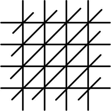
The issue with the above example is that it is really a 2-dimensional configuration, whereas we really want to ask a 3-dimensional question. One way to make the problem much more interesting is only count “truly 3-dimensional” intersection points.
Given a collection of lines in space, we define a joint to be a point that is contained in three of our lines and not all lying on the same plane.
Joints problem. What is the maximum number of joints that can be formed by L lines in 3-dimensional space?
The joints problem was raised in early 1990’s, and it turned out to be a very interesting problem! Besides its intrinsic interest as a combinatorial geometry problem, it also caught the attention of analysts as the joints problem is connected to the Kakeya problem, a central problem in analysis (this connection was popularized by Wolff).
Here are some examples of configurations of lines that have a lot of joints.
Example 1. The easiest example to visualize is by considering a \(k \times k \times k\) grid of lines, which has \(L = 3k^2\) lines and \(J = k^3 = (L/3)^{3/2}\) joints:
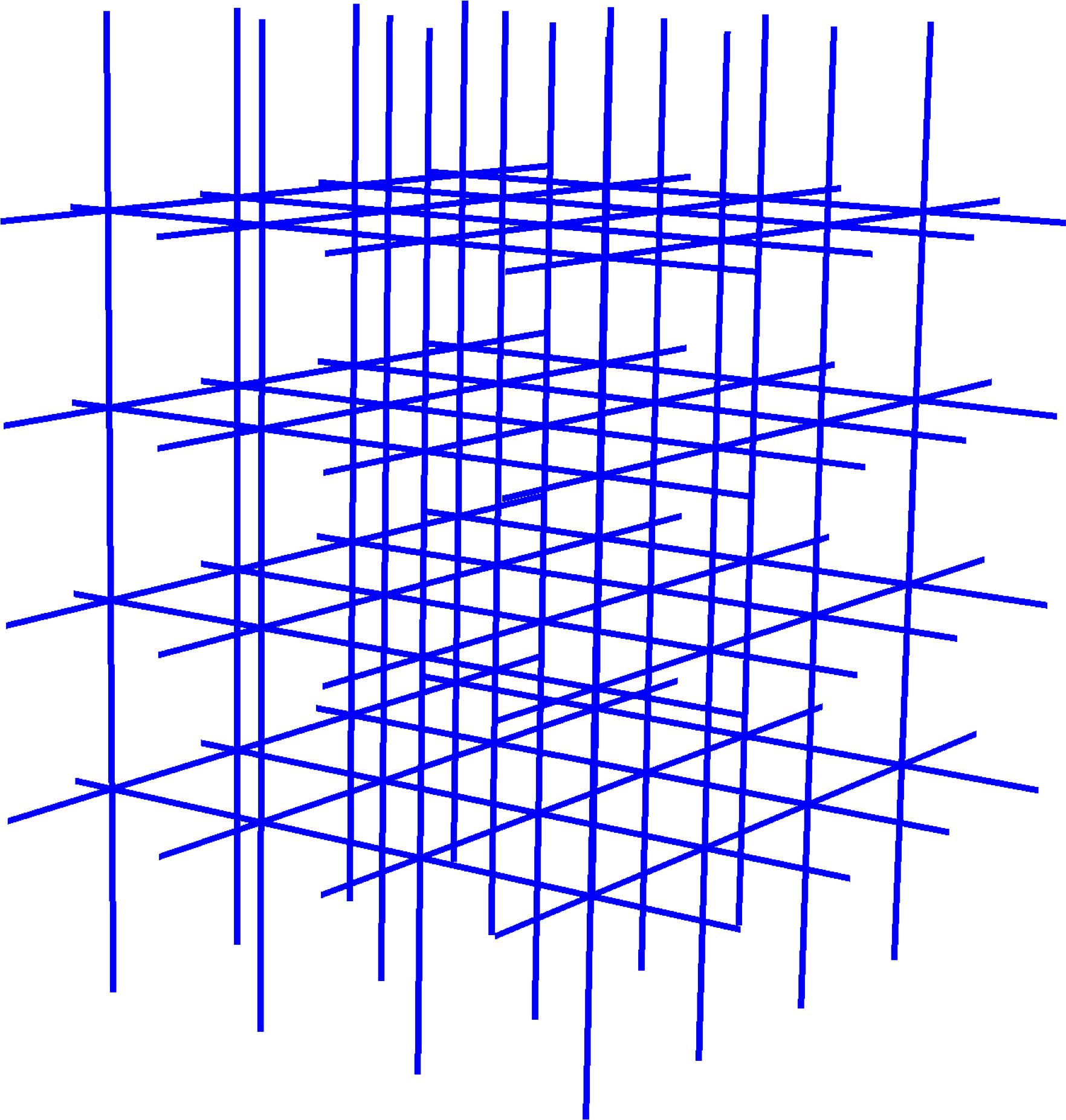
Example 2. Actually, there is another example that has even more joints (by a constant factor). Think about a tetrahedron, formed by 4 faces (planes), and whose edges form 6 lines, and the vertices form 4 joints. We can generalize the tetrahedron example by taking k generic planes in space, and have the planes pairwise intersect to make \(L = \binom{k}{2}\) lines, and triplewise intersect to make \(J = \binom{k}{3}\) joints. (This example appeared in the original paper on the joints problem.)
In both examples, the number of joints is \(\Theta(L^{3/2})\). A matching upper bound on the number of joints turned out to be much less obvious. A stunning breakthrough took place in 2008 when Guth and Katz proved an \(O(L^{3/2})\) upper bound on the number of joints in using the polynomial method. Their solution was partly inspired by Dvir’s stunning solution to the finite field Kakeya problem, and it was also a precursor to Guth and Katz’s subsequent celebrated solution of the Erdős distinct distances problem.
Larry Guth conjectured in his book The Polynomial Methods in Combinatorics that the second example above is best possible. I first learned about this very nice conjecture as a graduate student in Guth’s class on the polynomial method.
The main result of our paper is a new improved upper bound on the joints problem, matching the constant in the second example above. More precisely, we prove that L lines in space make at most \(\frac{\sqrt{2}}{3}L^{3/2}\) joints, thereby confirming Guth’s conjecture up to a \(1+o(1)\) factor. Our results also hold in arbitrary dimensions and over arbitrary fields.
It was quite unexpected to us that such a tight bound can even be proved, especially given how long it took just to obtain an upper bound of the right order of magnitude on the joints problem. In pretty much all other classical problems in incidence geometry (i.e., the Szemerédi–Trotter theorem), the optimal constant factor is not known. In fact, our result might be the first one in incidence geometry that obtains a tight constant factor.
Equiangular lines with a fixed angle
July 30, 2019
I’m happy to announce our new paper Equiangular lines with a fixed angle joint with four MIT coauthors: Zilin Jiang, Jonathan Tidor, Yuan Yao, and Shengtong Zhang.
Zilin is an Instructor (postdoc), Jonathan is my PhD student who just finished his second year, and Yuan and Shengtong are undergraduates who just finished their second and first respective years.
Our paper solves a longstanding problem in discrete geometry concerning equiangular lines, which are configurations of lines in space that are pairwise separated by the same angle. How many such lines can exist simultaneously in a given dimension?
We determine, for every fixed angle, the maximum number of equiangular lines with the given angle in high dimensions.
Our paper builds on a long sequence of earlier ideas. There were some important progress on this problem by Igor Balla, Felix Dräxler, Peter Keevash, and Benny Sudakov, as featured in this earlier Quanta Magazine article written for a lay audience.
In the end we finished off the problem in a clean and crisp manner, in a 10-page paper with a self-contained proof.
It has been known that the study of equiangular lines is closed linked to spectral graph theory, which seeks to understand graphs via their spectrum (i.e., eigenvalues). We prove our main result via a new insight in spectral graph theory, namely that a bounded degree graph must have sublinear second eigenvalue multiplicity.
Impartial digraphs
June 27, 2019
I just finished a new paper, Impartial digraphs, coauthored with Yunkun Zhou, who just completed his undergraduate studies at MIT and will be moving to Stanford to start his PhD this fall.
The problem (along with the conjecture that we proved) was proposed by Jacob Fox, Hao Huang, and Choongbum Lee. Ron Graham had also told me about this problem with much enthusiasm during tea time one afternoon at the Berkeley Simons Institute a couple of years ago, after learning about it from Jacob.
I really enjoyed working on this paper with Yunkun. The problem is natural and simple to state, the answer appears somewhat unexpected (at least initially), and the solution ended up being quite tricky yet clean, employing a variety of tools in combinatorics, ranging from analytic methods (graph limits), algebraic considerations (polynomial identities and factorization), as well basic combinatorial techniques such as bijections.
We are going to talk about directed graphs (which graph theorists like to abbreviate as digraphs). These are graphs where every edge is given an orientation.
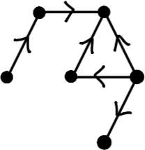
A tournament is a directed graph where there is a directed edge between every pair of vertices (think of it as recording the outcome of a round-robin tournament where every player plays against every other player).
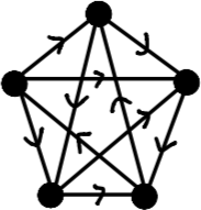
Given a directed graph H (think of it as a pattern), we can ask: how many different copies of the pattern H appear in a given tournament?
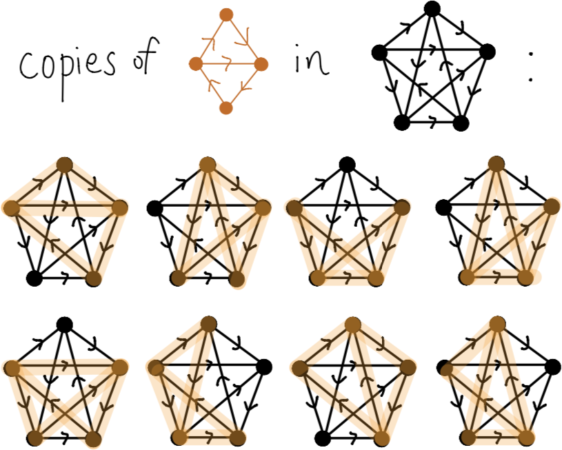
Look at the following 4-vertex tournament H. It has the following curious property: all tournaments of a fixed size contains the same number of copies of H, no matter how the edges in the tournament are oriented.
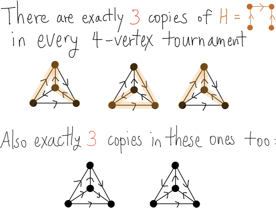
Hmm, why is this true? And are there other directed graphs H with the same property, namely that all tournaments of a given size contain the same number of copies of H?
In the good old mathematical tradition, we came up with a name for directed graphs H with this curious property: we called them impartial (as in: impartial judges of a tournament).
Okay. So why is the above directed graph impartial? Are there any other impartial directed graphs? What are all the impartial directed graphs?
Here is a simple example of an impartial digraph:
Here is another one:
Indeed, given any 10-vertex tournament, we can count the number of copies of the first edge (it doesn’t depend on the tournament), and then count the number of copies of the second edge among the remaining 8 vertices (it still doesn’t depend on the tournament).
Once these two edges are placed in a tournament, there are two ways to join their tips, but they result in identical patterns (one flipped from the other):
It must then follow that this directed graph is impartial as well:
We can follow the same logic and continue this procedure, iterate, and build up even larger impartial directed graphs. Each step, take two copies of the previous tree (keeping the same edge orientations), and then add a new edge between a twin pair of vertices.
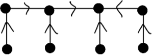
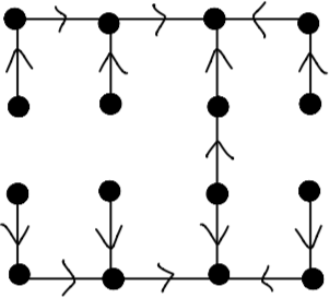
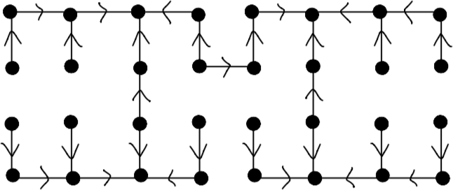
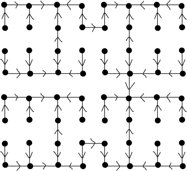
We call any directed graph that can building up as above a recursively bridge-mirrored tree.
The same argument as earlier shows that every recursively bridge-mirrored tree is impartial.
Are there other impartial digraphs? Did we miss any?
It turns out, there are actually no others. We have found them all, and that is the main result of our paper:
Theorem. A directed graph is impartial if and only if every component is recursively bridge-mirrored trees.
Just a word about how about this problem is related to a bigger picture. It is related to a number of other graph homomorphism inequalities that are central in extremal graph theory. It can be considered as the “equality case” for a directed analog of an open problem known as Sidorenko’s conjecture. See our paper for some further discussions and open problems.
A reverse Sidorenko inequality
September 26, 2018
Together with undergraduates Ashwin Sah, Mehtaab Sawhney, and David Stoner (the same team that proved Kahn’s conjecture on independent sets that I blogged about earlier, we are excited to announce our new paper A reverse Sidorenko inequality. This paper solves several open problems concerning graph colorings and homomorphisms, including one of my favorite problems regarding maximizing the number of q-colorings in a d-regular graph. I had previously blogged about some of these problems.
It has been truly a pleasure working with Ashwin, Mehtaab, and David on this project. I have learned so much from them.
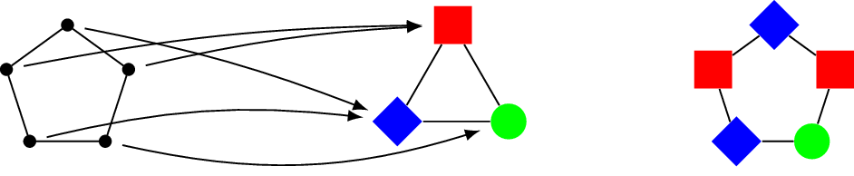
Here are some highlights of our new results.
1. Graph colorings.
Among d-regular graphs, which graph has the most number of proper q-colorings, exponentially normalized by the number of vertices of G?
We show that the extremal graph is the complete bipartite graph \(K_{d,d}\) (or disjoint unions thereof, as taking disjoint copies does not change the quantity due to the normalization).
2. Graph homomorphisms.
Among d-regular graphs, which triangle-free graph G has the most number of homomorphisms into a fixed H, again exponentially normalized by the number of vertices of G?
We show that the extremal graph G is the complete bipartite graph \(K_{d,d}\).
The triangle-free hypothesis on G is best possible in general. For certain specific H, such as \(K_q\), corresponding to proper q-colorings as earlier, the triangle-free hypothesis can be dropped. It remains a wide open problem to determine for which H can one drop the triangle-free hypothesis on G.
3. Partition functions of Ferromagnetic spin models.
Among d-regular graphs, which graph maximizes the log-partition function per vertex of a given Ferromagnetic spin model (e.g., Ising model)?
We show that the extremal graph is the clique \(K_{d+1}\).
For each setting, we establish our results more generally for irregular graphs as well, similar to our earlier work on independent sets.
Our results can be interpreted as a reverse form of the inequality in Sidorenko’s conjecture, an important open problem in graph theory stating a certain positive correlation on two-variable functions.
One can also view our results as a graphical analog of the Brascamp–Lieb inequalities, a central result in analysis.
This paper resolves one of my favorite open problems on this topic (the number of graph colorings). It also points us to many other open problems. Let me conclude by highlighting one of them (mentioned in #2 earlier). I’ll state it in a simpler form for d-regular graphs, but it can be stated more generally as well.
Open problem. Classify all H with the following property: among d-regular graphs G, the number of homomorphisms from G to H, exponentially normalized by the number of vertices of G, is maximized by \(G = K_{d,d}\).
Our results show that \(H = K_q\) works, even when some of its vertices are looped. Generalizing this case, we conjecture that all antiferromagnetic models H have the same property (though we know that this would not be the complete class, even if true).
The number of independent sets in an irregular graph
May 12, 2018
I am excited to announce our new paper, The number of independent sets in an irregular graph, coauthored with these three amazing collaborators:


Ashwin is a freshman at MIT, Mehtaab is a sophomore at MIT, and David is a junior at Harvard.
The paper solves a conjecture made by Jeff Kahn in 2001 concerning the number of independent sets in a graph.
An independent set of a graph is a subset of vertices with no two adjacent.
Since many problems in combinatorics can be naturally phrased in terms of independent sets in a graph or hypergraph, getting good bounds on the number of independent sets is a problem of central importance.
Instead of giving the exact statement of the conjecture (now theorem), which you can find in the abstract of our paper, let me highlight a specific instance of a problem addressed by the theorem:
Question. Consider the family of graphs with no isolated vertices and
- exactly a third of the edges have degree 3 on both endpoints, and
- a third of the edges have degree 4 on both endpoints,
- the remaining third of the edges have degree 3 on one endpoint and degree 4 on the other endpoint.
What is the smallest constant c such that every n-vertex graph satisfying the above properties has at most \(c^n\) independent sets?
In other words, letting \(i(G)\) denote the number of independent sets and \(v(G)\) the number of vertices of \(G\), maximize the quantity \(i(G)^{1/v(G)}\) over all graphs G in the above family.
(See the end of this post for the answer)
In summer 2009, as an undergraduate participating in the wonderful Research Experience for Undergraduates (REU) run by Joe Gallian in Duluth, MN, I learned about Kahn’s conjecture (somewhat accidentally actually, as I was working on a different problem that eventually needed some bounds on the number of independent sets, and so I looked up the literature and learned, slightly frustratingly at the time, that it was an open problem). It was on this problem that I had written one of my very first math research papers.
I had been thinking about this problem on and off since then. A couple years ago, Joe Gallian invited me to write an article for a special issue of the American Mathematical Monthly dedicated to undergraduate research (see my previous blog post on this article), where I described old and new developments on the problem and collected a long list of open problems and conjectures on the topic (one of them being Kahn’s conjecture).
This spring, I had the privilege with working with Ashwin, Mehtaab, and David, three energetic and fearless undergraduate students, finally turning Kahn’s conjecture into a theorem. Fearless indeed, as our proof ended up involving quite a formidable amount of computation (especially for such an innocent looking problem), and my three coauthors deserve credit for doing the heavy-lifting. I’ve been told that there had been many late night marathon sessions in an MIT Building 2 classroom where they tore apart one inequality after another.
This is certainly not the end of the story, as many more interesting problems on the subject remain unsolved—my favorite one being the analogous problem for colorings, e.g., instead of counting the number of independent sets, how about we count the number of ways to color the vertices of the graph with 3 colors so that no two adjacent vertices receive the same color? (See my previous blog post for some more discussion.)
Anyway, here is the the answer to the question above. The number of independent sets in an n-vertex graph satisfying the above properties is at most \(c^n\), where the optimal constant for c is \(15^{4/63} \times 23^{1/21} \times 31^{1/28} = 1.558\dots\), or, more helpfully, the maximum is attained by the following graph (in general, the theorem says that the maximizer is always a disjoint union of complete bipartite graphs):